1. Load Packages
library(tidyverse)
library(gt)
library(DT)
library(moments)
library(sf)
library(leaflet)
library(leaflet.extras)
library(leafgl)
2. Import Cleaned Data
cleaned_rides <- readRDS("Data/cleaned_rides.RDS")
3. Ride origins and destinations
#Data needs to be binned https://search.r-project.org/CRAN/refmans/leaflet.extras2/html/addHexbin.html

member_endlatlng <- cleaned_rides %>%
  filter(member_casual == 'member') %>%
  select(end_lat, end_lng)
member_endlatlng_pts <- st_as_sf(member_endlatlng,
                                 coords = c("end_lng", "end_lat"), crs = 4326)

casual_endlatlng <- cleaned_rides %>%
  filter(member_casual == 'casual') %>%
  select(end_lat, end_lng)
casual_endlatlng_pts <- st_as_sf(casual_endlatlng,
                                 coords = c("end_lng", "end_lat"), crs = 4326)

member_startlatlng <- cleaned_rides %>%
  filter(member_casual == 'member') %>%
  select(start_lat, start_lng)
member_startlatlng_pts <- st_as_sf(member_startlatlng,
                                 coords = c("start_lng", "start_lat"), crs = 4326)

casual_startlatlng <- cleaned_rides %>%
  filter(member_casual == 'casual') %>%
  select(start_lat, start_lng)
casual_startlatlng_pts <- st_as_sf(casual_startlatlng,
                                 coords = c("start_lng", "start_lat"), crs = 4326)

endlatlng <- cleaned_rides %>%
  select(end_lat, end_lng, member_casual)
endlatlng_pointmap_gl <- endlatlng %>%
  leaflet(options = leafletOptions(preferCanvas = TRUE)) %>%
  addProviderTiles("Esri.WorldGrayCanvas",
                   options = providerTileOptions(pdateWhenZooming = FALSE,
                                                 updateWhenIdle = TRUE)) %>%
  setView(lng = -87.65, lat = 41.9, zoom = 10) %>%
  addGlPoints(data = member_endlatlng_pts, fillColor = "#4e7dcc",
              radius = 4, fillOpacity = 0.9, group = "Member (End Station)") %>%
  addGlPoints(data = casual_endlatlng_pts, fillColor = "#c65e57",
              fillOpacity = 0.9, radius = 4, group = "Casual (End Station)") %>%
  addGlPoints(data = member_startlatlng_pts, fillColor = "#619CFF",
              radius = 4, fillOpacity = 0.9, group = "Member (Start Station)") %>%
  addGlPoints(data = casual_startlatlng_pts, fillColor = "#F8766D",
              fillOpacity = 0.9, radius = 4, group = "Casual (Start Station)") %>%
  addLayersControl(
    overlayGroups = c("Member (Start Station)", "Casual (Start Station)",
                      "Member (End Station)", "Casual (End Station)"),
    options = layersControlOptions(collapsed = FALSE))
endlatlng_pointmap_gl
#Top Stations (Start)
start_station_rank <- cleaned_rides %>%
  select(station_name = start_station_name, member_casual) %>%
  group_by(member_casual) %>%
  count(station_name) %>%
  pivot_wider(names_from = member_casual, values_from = n)

#Top Stations (End)
end_station_rank <- cleaned_rides %>%
  select(station_name = end_station_name, member_casual) %>%
  group_by(member_casual) %>%
  count(station_name) %>%
  pivot_wider(names_from = member_casual, values_from = n)

#Top Stations (Combined)
all_station_rank <- full_join(start_station_rank, end_station_rank, by = "station_name") %>%
  mutate(member_trips=member.x+member.y) %>%
  mutate(casual_trips=casual.x+casual.y) %>%
  mutate(member_rank = row_number(-member_trips)) %>%
  mutate(casual_rank = row_number(-casual_trips)) %>%
  mutate(total_trips = casual_trips + member_trips) %>%
  select(station_name,casual_trips, casual_rank, member_trips, member_rank,
         total_trips) %>%
  arrange(desc(total_trips))

datatable(all_station_rank, colnames = c("Station Name", "Visits (Casual)",
                                         "Rank (Casual)", "Visits (Member)",
                                         "Rank (Member)", "Visits (Total)"))
#all_station_rank <- full_join(start_station_rank, end_station_rank, by = "station_name") %>%
#  mutate(total_start=casual.x + member.x) %>%
#  mutate(total_end=casual.y + member.y) %>%
#  arrange(desc(total_start+total_end))
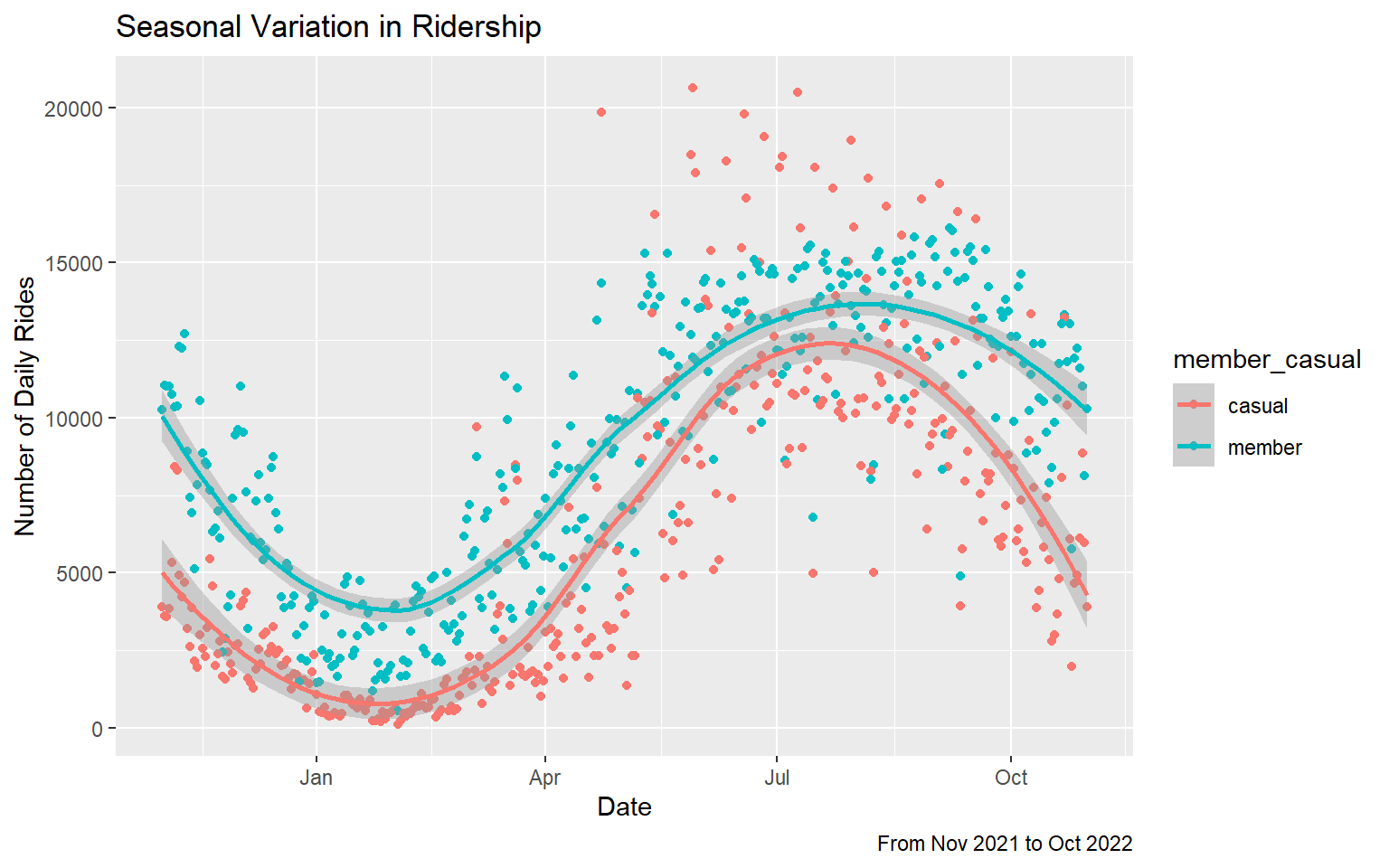
4. Seasonal ridership patterns
year_table <- cleaned_rides %>%
  select(started_at, member_casual) %>%
  group_by(member_casual) %>%
  count(date = date(started_at)) %>%
  arrange(-n)

year_plot <- ggplot(year_table, mapping = aes(x = date, y = n, color = member_casual)) +
  geom_point() +
  geom_smooth() +
  scale_x_date(date_labels = "%b")+
  labs(x = "Date", y = "Number of Daily Rides",
       title = "Seasonal Variation in Ridership",
       caption = "From Nov 2021 to Oct 2022")
year_plot
month_table <- xtabs(~member_casual+month(cleaned_rides$started_at), data=cleaned_rides)
colnames(month_table) <- month.name
prop_month_table <- prop.table(month_table)
prop_month_table <- round(prop_month_table, 3)
prop_month_table <- addmargins(prop_month_table)
prop_month_table
             month(cleaned_rides$started_at)
member_casual January February March April   May  June  July August September
       casual   0.003    0.004 0.016 0.022 0.049 0.064 0.070  0.062     0.051
       member   0.015    0.016 0.034 0.043 0.062 0.070 0.072  0.074     0.070
       Sum      0.018    0.020 0.050 0.065 0.111 0.134 0.142  0.136     0.121
             month(cleaned_rides$started_at)
member_casual October November December   Sum
       casual   0.036    0.019    0.012 0.408
       member   0.061    0.044    0.031 0.592
       Sum      0.097    0.063    0.043 1.000
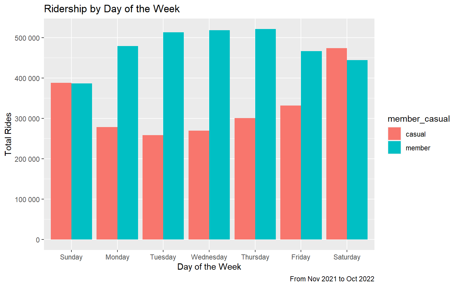
5. Rides by day of the week
week_plot <- ggplot(cleaned_rides, aes(fill = member_casual, x = day_of_week))+
  geom_bar(position = "dodge", stat = "count") +
  scale_y_continuous(labels = scales::label_number())+
  labs(y = "Total Rides", x = "Day of the Week",
       title = "Ridership by Day of the Week",
       caption = "From Nov 2021 to Oct 2022")

week_plot
day_table <- xtabs(~member_casual+day_of_week, data=cleaned_rides)
prop_day_table <- prop.table(day_table)
prop_day_table <- round(prop_day_table, 3)
prop_day_table <- addmargins(prop_day_table)
prop_day_table
             day_of_week
member_casual Sunday Monday Tuesday Wednesday Thursday Friday Saturday   Sum
       casual  0.069  0.050   0.046     0.048    0.053  0.059    0.084 0.409
       member  0.069  0.085   0.091     0.092    0.093  0.083    0.079 0.592
       Sum     0.138  0.135   0.137     0.140    0.146  0.142    0.163 1.001
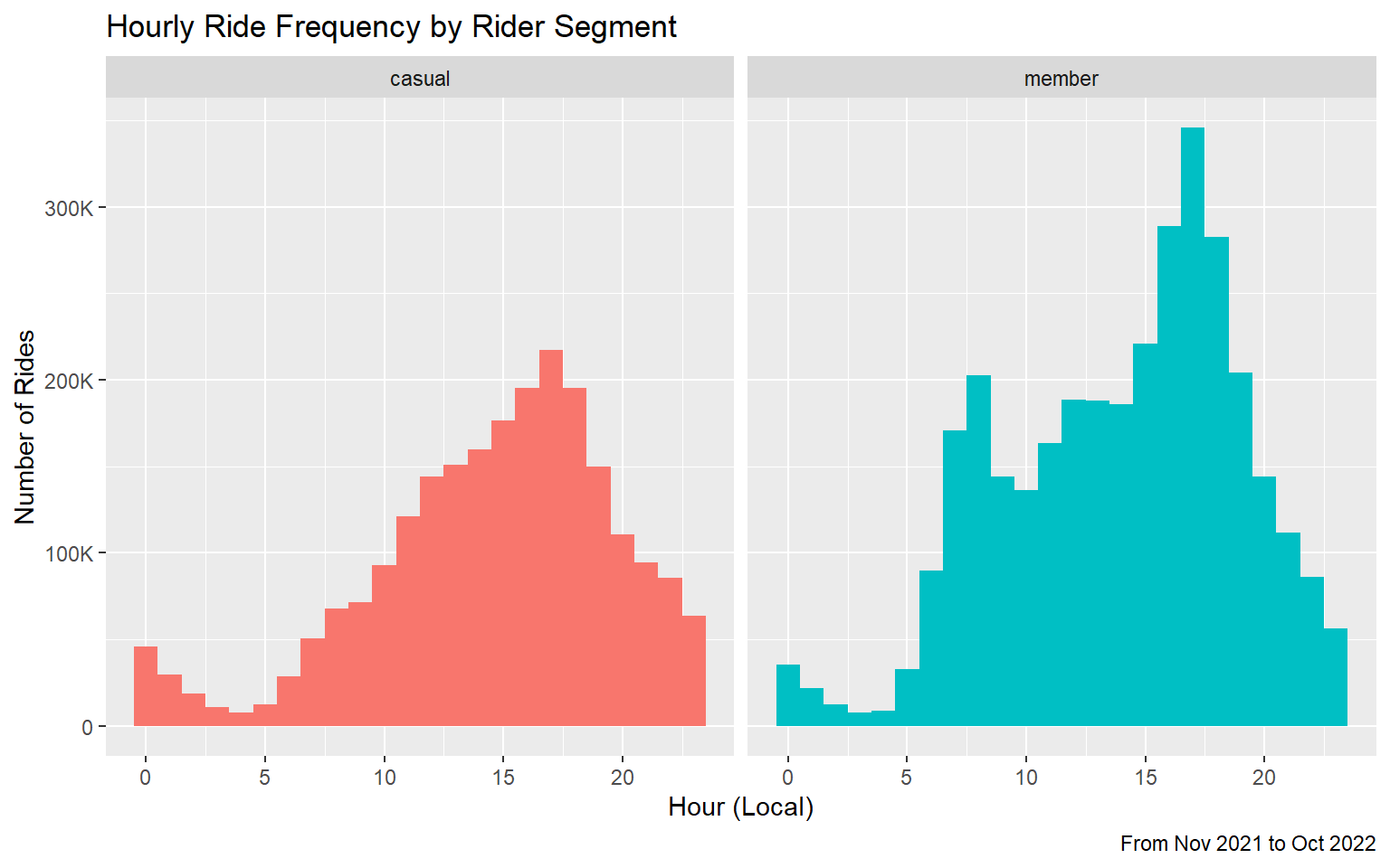
6. Rides by time of Day
day_plot <- ggplot(cleaned_rides) +
  geom_histogram(mapping = aes(x=hour(started_at), fill = member_casual),
                 binwidth = 1)+
  scale_y_continuous(labels = scales::label_number_si())+
  labs(x = "Hour (Local)", y = "Number of Rides",
       title = "Hourly Ride Frequency by Rider Segment",
       caption = "From Nov 2021 to Oct 2022") +
  guides(fill = 'none') +
  facet_wrap(~member_casual)
day_plot
hour_table <- xtabs(~member_casual+format(started_at, "%H"), data=cleaned_rides)
prop_hour_table <- prop.table(hour_table)
prop_hour_table <- round(prop_hour_table, 3)
prop_hour_table <- addmargins(prop_hour_table)
prop_hour_table
             format(started_at, "%H")
member_casual    00    01    02    03    04    05    06    07    08    09    10
       casual 0.008 0.005 0.003 0.002 0.001 0.002 0.005 0.009 0.012 0.013 0.016
       member 0.006 0.004 0.002 0.001 0.002 0.006 0.016 0.030 0.036 0.026 0.024
       Sum    0.014 0.009 0.005 0.003 0.003 0.008 0.021 0.039 0.048 0.039 0.040
             format(started_at, "%H")
member_casual    11    12    13    14    15    16    17    18    19    20    21
       casual 0.021 0.026 0.027 0.028 0.031 0.035 0.039 0.035 0.027 0.020 0.017
       member 0.029 0.033 0.033 0.033 0.039 0.051 0.061 0.050 0.036 0.026 0.020
       Sum    0.050 0.059 0.060 0.061 0.070 0.086 0.100 0.085 0.063 0.046 0.037
             format(started_at, "%H")
member_casual    22    23   Sum
       casual 0.015 0.011 0.408
       member 0.015 0.010 0.589
       Sum    0.030 0.021 0.997
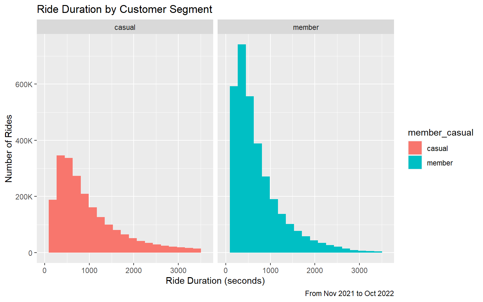
7. Ride duration
duration_histogram <- ggplot(cleaned_rides, aes(ride_duration, fill = member_casual)) +
  geom_histogram(binwidth = 180) +
  xlim(0,3600) +
  scale_y_continuous(labels  = scales::label_number_si())+
  labs(x = "Ride Duration (seconds)", y = "Number of Rides",
       title = "Ride Duration by Customer Segment",
       caption = "From Nov 2021 to Oct 2022") +
  facet_wrap(~member_casual)
duration_histogram
duration_table <- cleaned_rides %>%
  group_by(member_casual) %>%
  summarize(q1 = quantile(ride_duration, 0.25),
            median = as.duration(median(as.numeric(ride_duration))),
            q3 = quantile(ride_duration, 0.75),
            IQR = as.duration(IQR(ride_duration)),
            skewness = skewness(ride_duration))
duration_table
# A tibble: 2 × 6
member_cas…¹ q1 median q3
<fct> <Duration> <Duration> <Duration>
1 casual 464s (~7.73 minutes) 805s (~13.42 minutes) 1474s (~24.57 minutes)
2 member 319s (~5.32 minutes) 541s (~9.02 minutes) 930s (~15.5 minutes)
# … with 2 more variables: IQR <Duration>, skewness <dbl>, and abbreviated
# variable name ¹member_casual
8. Rideable Type
rideable_df <- cleaned_rides %>%
group_by(member_casual, rideable_type) %>%
count(rideable_type)
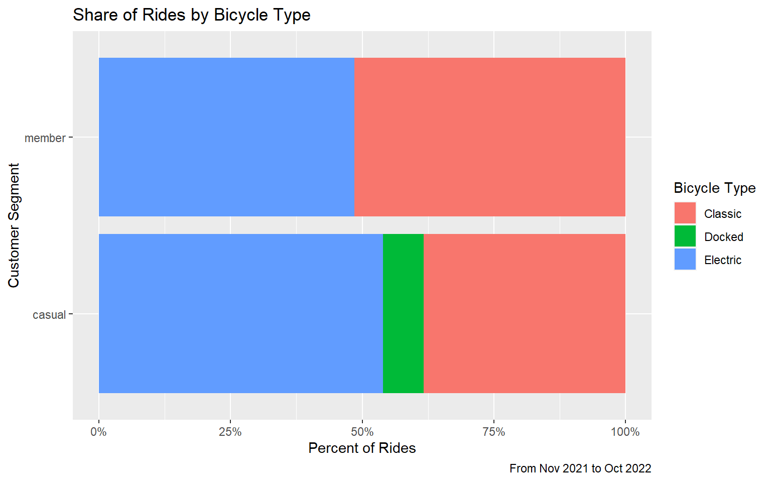
rideable_plot <- ggplot(rideable_df) +
geom_col(mapping = aes(x = member_casual, y = n, fill = rideable_type), position =
"Fill") +
labs(x = "Customer Segment", y = "Percent of Rides",
title = "Share of Rides by Bicycle Type", caption = "From Nov 2021 to Oct 2022") +
scale_fill_discrete(name = "Bicycle Type",
labels = c("Classic", "Docked", "Electric")) +
scale_y_continuous(name=waiver(), labels = scales::percent) +
coord_flip()
rideable_plot
rideable_table <- table(cleaned_rides$rideable_type, cleaned_rides$member_casual)
rideable_table
                 casual  member
  classic_bike   882197 1713853
  docked_bike    177938       0
  electric_bike 1240624 1616519
1240624/(882197+177938+1240624)#53.9%
[1] 0.5392238
1616519/(1616519+1713853)#48.5%
[1] 0.4853869